How To:
- Highlight the range of cells that you want to format.
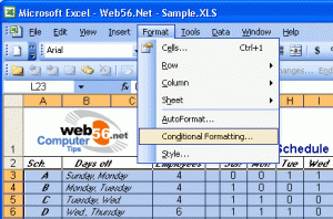
- From the drop down menu select Format -> Conditional Formatting this will bring up the the Conditional Formatting dialog box.

3. From the first drop down option in the Conditional Formatting dialog box select Formula is, then in the second box type in the formula =MOD(ROW(),2)=0 in the second box.
4. From the Conditional Formatting dialog box click on the Format button to bring up the Format Cells dialog box.
5. By clicking on the patterns tab you can now select a color for the background of the alternate rows. Make sure you choose a light color which will allow you to see the content of the cells. You can do any other formatting you would like which is available here such as font, font type, color etc.

6. Now that we are happy with our selections we simply click OK to accept the formatting options your spreadsheet now has every other row highlited.
The great part about this is that the formatting stays in every other row wether you delete a row, insert a row etc.
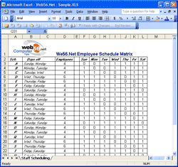
BEFORE

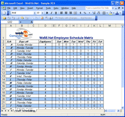
AFTER


